GENeSYS-MOD Weather Timeseries & Renewable Potential Tool
The timeseries script creates the capacity factors for solar PV, wind (onshore and offshore) and heat pumps, as well as residential heating and cooling demand. In addition, it can derive GIS-based renewable energy potentials (utility-scale PV, onshore wind, rooftop PV and offshore wind) from land-cover and protected-area data. It uses functions from atlite and the ERA5 weather dataset, which is downloaded and transformed locally. This section provides a step-by-step guide on how to use the script and change its settings to fit a specific case study.
Requirements
Python: If you don’t have Python installed on your system already you can download it here: https://www.python.org/downloads/
Jupyter Notebook: You will need a Jupyter Notebook to run the script. You can directly install Jupyter Notebook by following the instructions here: https://jupyter.org/install or use Anaconda, which provides a bundled environment manager and Jupyter Notebook setup: https://www.anaconda.com/download
Packages: To use this script, you will also need to have the following packages installed:
numpy
matplotlib
seaborn
pandas
geopandas
scikit-learn
cartopy
xarray
atlite
rasterio (for the GIS-based potential analysis)
You can install all the necessary packages with the following command:
pip install numpy matplotlib seaborn pandas geopandas scikit-learn cartopy xarray atlite rasterio
API key: In addition, in order to be able to load the ERA5 cutouts, you need an API key. To activate the API key, follow the instructions at https://cds.climate.copernicus.eu/how-to-api
Set Up
The timeseries script, along with all necessary data files and functions, can be found here: https://github.com/GENeSYS-MOD/GENeSYS_MOD.tools/tree/main/GIS_%26_Timeseries_Tool
You can either clone the repository or download the files directly to your computer. Be sure to note the location where you save the files.
Two notebooks are provided:
GENeSYS-MOD_RES_Tool.ipynb— the main notebook. It ships with a small, self-contained example for Germany (single day, coarse resolution) including a region polygon, the German Exclusive Economic Zone (EEZ) and a bathymetry subset, so it runs end-to-end with only a CDS API key.GENeSYS-MOD_RES_Tool_DE.ipynb— a variant of the original country-based workflow, where regions are selected via ISO country codes (e.g.DE) and the CORINE land cover is used for the potential analysis.
All re-usable logic lives in functions.py; the notebooks only set paths and
parameters. The functions are region-agnostic: to study a different country or
set of regions, only the input files and parameter cells need to change.
Configuration
The configuration cell at the top of the notebook controls the study setup:
geo_file— a GeoJSON with the region polygons to analyse (aregioncolumn, one row per region). The example shipsexample_germany.geojsonwith a single “Germany” region. Results are produced per region in this file.offshore_file/bathymetry_file— an EEZ polygon and a bathymetry grid for the offshore analysis. Setting both toNonedisables all offshore steps; the notebook will skip them gracefully.timeframe— e.g."2018","2018-01"or"2018-01-01". Start with a single day to verify the setup before downloading a full year.filename— name for the downloaded cutout; change it for every new region or year.regions— optional subset of region names from thegeo_file; an empty list uses all regions.
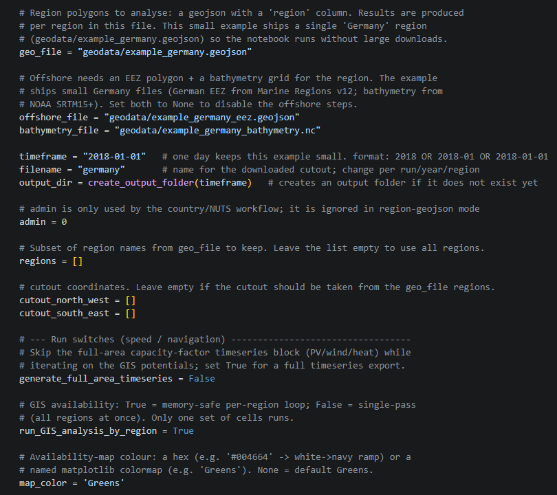
Two run switches help navigating the notebook without accidentally triggering slow computations:
generate_full_area_timeseries— whenFalse(default), the full-area capacity-factor cells (PV, wind, heat) are skipped. Set it toTruefor a complete timeseries export.run_GIS_analysis_by_region— switches between the memory-safe per-region potential analysis (True, recommended) and the single-pass variant that processes all regions at once.
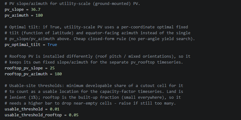
The solar-panel orientation can be set globally (pv_slope, pv_azimuth)
or computed per coordinate by enabling pv_optimal_tilt: each grid cell then
uses an optimal fixed tilt derived from its latitude with an equator-facing
azimuth. Rooftop PV uses its own, separate orientation settings, since roof
geometry differs from utility-scale installations.
The spatial resolution of the cutout is set via dx_step and dy_step
(in degrees):

Cutout preparation
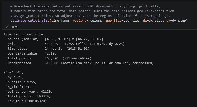
Before any download, the cell calling estimate_cutout_size prints the
expected grid dimensions, the number of hourly steps and the total number of
data points for the chosen region, timeframe and resolution. Check this first —
a full-year, fine-resolution cutout over a large region can reach several
gigabytes.
get_cutout then downloads and prepares the ERA5 cutout. The download is
resilient: every data chunk retrieved from the Climate Data Store is cached
locally (cutouts/era5_cache), so an interrupted run resumes from the cache
instead of re-downloading. Incomplete or corrupted cutouts are detected and
rebuilt automatically. Once a cutout has been fully prepared it is reused on
every subsequent run.
Note
Downloading the weather data can take a significant amount of time, depending on the size of the region and the timeframe selected. It is recommended to use a device with ample system memory (at least 24 GB of RAM for the full European dataset) and a stable internet connection.
Capacity-factor timeseries
Running the timeseries section produces hourly capacity factors per region for:
solar PV (fixed tilt or per-coordinate optimal tilt, plus tracking variants),
onshore wind,
offshore wind, split by water depth into shallow, transitional (both fixed-bottom foundations) and deep (floating) sites,
heat-pump coefficients of performance and heating/cooling demand profiles.
For PV and onshore wind, the sites within each region are split into three
quality categories based on the regional 30th and 70th percentile of the annual
capacity factor: inf (below average), avg and opt (above average).
One CSV per technology and category is written to the output folder.
GIS-based renewable potentials
The second part of the notebook estimates how much land (and sea) area is actually available for renewable installations, and converts it into capacity potentials.
Exclusion layers. Land availability is derived from a categorical land-cover raster and optional protected-area data. For Europe, the CORINE Land Cover (100 m resolution) is the standard choice; protected areas can be taken from the WDPA or a national dataset, optionally filtered to strict IUCN categories. The notebook defines which land-cover classes are excluded (e.g. artificial surfaces, arable land, forests, wetlands and water bodies) and which remain available (e.g. pastures, natural grassland, shrub land). The rooftop-PV potential uses the urban fabric classes as a proxy for built-up area. All class lists are plain Python lists in the notebook and can be adjusted to the land-availability assumptions of a study.
An additional, separate exclusion set can be supplied for onshore wind only (for example stricter protection classes or municipalities with wind restrictions), in which case wind uses its own availability layer while PV keeps the general one.
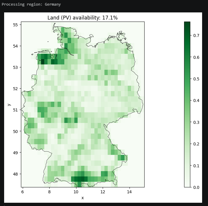
Availability and potentials. The memory-safe driver processes one region at
a time — important for large rasters — and produces, per region: the available
share of every grid cell, suitable areas and capacity potentials for
utility-scale PV, onshore wind and rooftop PV (using configurable capacity
densities in MW/km² and land-availability factors), and a combined CSV. PV and
onshore-wind potentials are additionally broken down into the inf/avg/
opt site-quality categories. Stitched availability maps across all regions
are plotted, with the headline number being the area-weighted mean availability;
the map colour can be customised via the map_color setting.
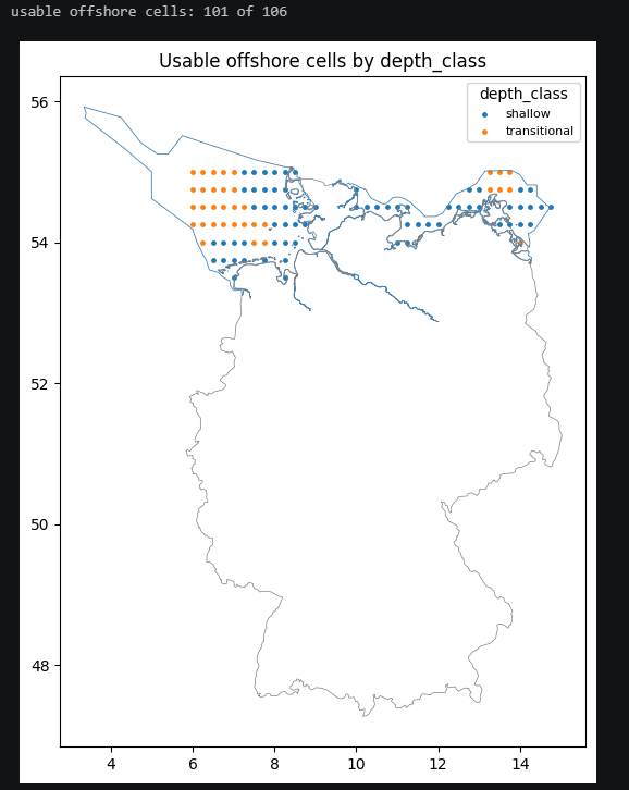
Offshore potentials. Offshore wind potential is computed from the EEZ cells per region and water-depth class. Marine protected areas or other no-build zones can be excluded by passing a vector file (e.g. a WDPA subset). Both the unconstrained (depth-only) and the constrained (“usable”) potential are written to separate CSV files for comparison.
Usable sites. The set of grid cells that pass the exclusion filters (“usable sites”) is exported with its availability share and site-quality category, and the capacity-factor timeseries can be recomputed for these usable sites only — providing timeseries that are consistent with the potential analysis. Maps of the usable onshore, rooftop and offshore sites are plotted at the end of the notebook.
Run Code and Use Output
After adjusting the settings, run the Jupyter Notebook cell by cell from top to bottom. Once the data processing is complete, the output folder contains:
hourly capacity-factor CSV files per technology, region and site category,
per-region and combined potential CSV files (areas in km², capacities in GW),
the usable-site coordinate lists,
the availability and site maps shown in the notebook.
Open these files and copy the columns into your desired hourly data file for further use. The notebook also displays a map of the cutout area and the means of all generated factors, allowing you to check for plausibility.